Introduction to vsn

Wolfgang Huber

Getting started

VSN is a method to preprocess microarray intensity data. This can be as simple as

library("vsn")
data("kidney")
xnorm = justvsn(kidney)

where kidney is an ExpressionSet object with unnormalised data and xnorm the resulting ExpressionSet with calibrated and glog$_2$-transformed data.

M = exprs(xnorm)[,1] - exprs(xnorm)[,2]

produces the vector of generalised log-ratios between the data in the first and second column.

VSN is a model-based method, and the more explicit way of doing the above is

fit = vsn2(kidney)
ynorm = predict(fit, kidney)

where fit is an object of class vsn that contains the fitted calibration and transformation parameters, and the method predict applies the fit to the data. The two-step protocol is useful when you want to fit the parameters on a subset of the data, e.g. a set of control or spike-in features, and then apply the model to the complete set of data¹. Furthermore, it enables further inspection of the fit object, e.g., for the purpose of quality assessment.

Besides ExpressionSets, there are also justvsn methods for AffyBatch objects from the affy package and RGList objects from the limma package. They are described in this vignette.

The so-called glog$_2$ (short for generalised logarithm) is a function that is like the logarithm (base 2) for large values (large compared to the amplitude of the background noise), but is less steep for smaller values. While the $\log_2$ function diverges to negative infinity at zero, the glog$_2$ function approximates a straight line of finite slope around 0². Differences between the transformed values are the generalised log-ratios. These are shrinkage estimators of the logarithm of the fold change. The usual log-ratio is another example for an estimator³ of log fold change. There is also a close relationship between background correction of the intensities and the variance properties of the different estimators. Please see Section @ref(sec:shrink) for more explanation of these issues.

How does VSN work? There are two components: First, an affine transformation whose aim is to calibrate systematic experimental factors such as labelling efficiency or detector sensitivity. Second, a glog$_2$ transformation whose aim is variance stabilisation.

An affine transformation is simply a shifting and scaling of the data, i.e. a mapping of the form $x\mapsto (x-a)/s$ with offset $a$ and scaling factor $s$. By default, a different offset and a different scaling factor are used for each column, but the same for all rows within a column. There are two parameters of the function vsn2 to control this behaviour: With the parameter strata, you can ask vsn2 to choose different offset and scaling factors for different groups (“strata”) of rows. These strata could, for example, correspond to sectors on the array⁴. With the parameter calib, you can ask vsn2 to choose the same offset and scaling factor throughout⁵. This can be useful, for example, if the calibration has already been done by other means, e.g., quantile normalisation.

Limitations

Other determinants of variance

The VSN transformation only addresses the dependence of the variance on the mean intensity. There may be important other factors influencing the variance, including gene-inherent properties, sample-inherent properties such as different tightness of transcriptional control in different conditions, or technical factors. These need to be addressed by other, more specialized models.

Numerical stability and convergence

VSN does not work for all possible inputs. If you encounter an error message like “L-BFGS-B needs finite values of ‘fn’”⁶, please check whether one of these problems is present:

• A bug in the code that does the preprocessing of the data that go in.
• A problem with data quality or experimental design, e.g., incompatible measurements assembled together into one input matrix.
• The noise or variance characteristics of the data are just not suitable for the VSN model.

Running VSN on data from a single two-colour array

The dataset kidney contains example data from a spotted cDNA two-colour microarray on which cDNA from two adjacent tissue samples of the same kidney were hybridised, one labeled in green (Cy3), one in red (Cy5). The two columns of the matrix exprs(kidney) contain the green and red intensities, respectively. A local background estimate⁷ was calculated by the image analysis software and subtracted, hence some of the intensities in kidney are close to zero or negative. In Figure @ref(fig:nkid-scp) you can see the scatterplot of the calibrated and transformed data. For comparison, the scatterplot of the log-transformed raw intensities is also shown. The code below involves some data shuffling to move the data into datasframes for ggplot.

library("ggplot2")
allpositive = (rowSums(exprs(kidney) <= 0) == 0)

df1 = data.frame(log2(exprs(kidney)[allpositive, ]),
                 type = "raw",
         allpositive = TRUE)
df2 = data.frame(exprs(xnorm),
                 type = "vsn",
         allpositive = allpositive)
df = rbind(df1, df2)
names(df)[1:2] = c("x", "y") 

ggplot(df, aes(x, y, col = allpositive)) + geom_hex(bins = 40) +
  coord_fixed() + facet_grid( ~ type)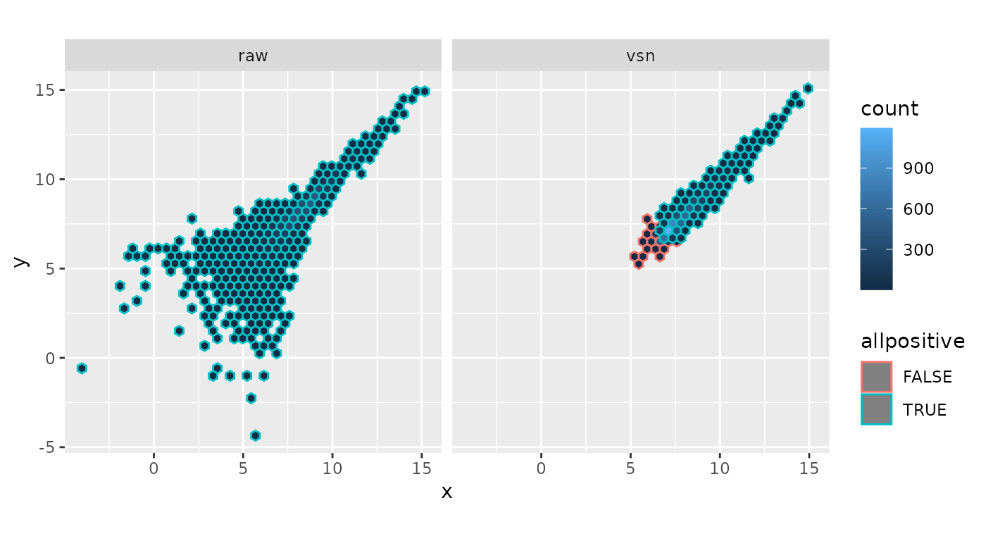

Scatterplots of the kidney example data, which were obtained from a two-color cDNA array by quantitating spots and subtracting a local background estimate. a) unnormalised and $\log_2$-transformed. b) normalised and transformed with VSN. Panel b shows the data from the complete set of 8704 spots on the array, Panel a only the 7806 spots for which both red and green net intensities were greater than 0. Those spots which are missing in Panel a are coloured in orange in Panel b.

To verify the variance stabilisation, there is the function meanSdPlot. For each feature $k=1,\ldots,n$ it shows the empirical standard deviation $\hat{\sigma}_k$ on the $y$-axis versus the rank of the average $\hat{\mu}_k$ on the $x$-axis.

$$\begin{equation} \hat{\mu}_k =\frac{1}{d} \sum_{i=1}^d h_{ki}\quad\quad \hat{\sigma}_k^2=\frac{1}{d-1}\sum_{i=1}^d (h_{ki}-\hat{\mu}_k)^2 \end{equation}$$

meanSdPlot(xnorm, ranks = TRUE)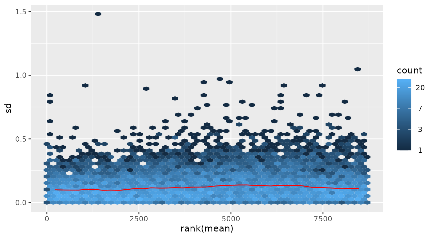

Standard deviation versus rank of the mean

meanSdPlot(xnorm, ranks = FALSE)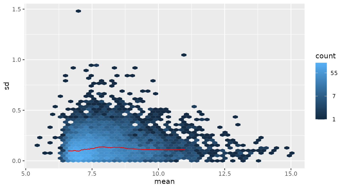 

Standard deviation versus mean

The red dots, connected by lines, show the running median of the standard deviation⁸. The aim of these plots is to see whether there is a systematic trend in the standard deviation of the data as a function of overall expression. The assumption that underlies the usefulness of these plots is that most genes are not differentially expressed, so that the running median is a reasonable estimator of the standard deviation of feature level data conditional on the mean. After variance stabilisation, this should be approximately a horizontal line. It may have some random fluctuations, but should not show an overall trend. If this is not the case, that usually indicates a data quality problem, or is a consequence of inadequate prior data preprocessing. The rank ordering distributes the data evenly along the $x$-axis. A plot in which the $x$-axis shows the average intensities themselves is obtained by calling the plot command with the argument ranks=FALSE; but this is less effective in assessing variance and hence is not the default.

The histogram of the generalized log-ratios:

hist(M, breaks = 100, col = "#d95f0e")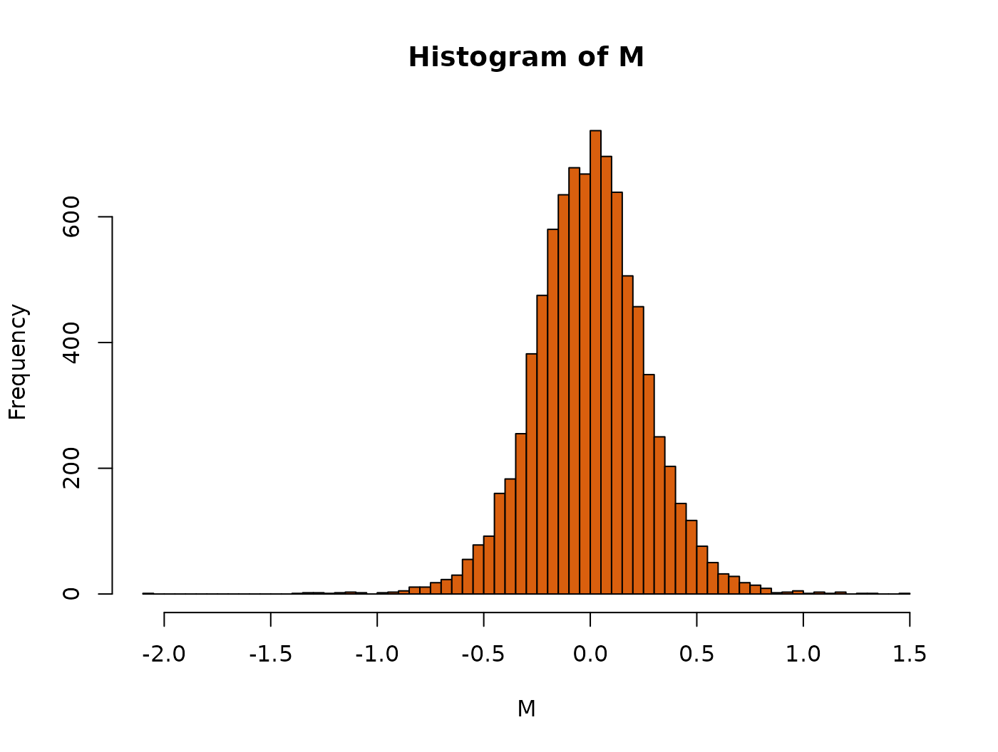

Histogram of generalised log-ratios for the kidney example data.

Running VSN on data from multiple arrays (“single colour normalisation”)

The package includes example data from a series of 8 spotted cDNA arrays on which cDNA samples from different lymphoma were hybridised together with a reference cDNA (Alizadeh et al. 2000).

data("lymphoma")
dim(lymphoma)

## Features  Samples 
##     9216       16

The 16 columns of the lymphoma object contain the red and green intensities, respectively, from the 8 slides.

pData(lymphoma)

##                      name    sample dye
## lc7b047.reference lc7b047 reference Cy3
## lc7b047.CLL-13    lc7b047    CLL-13 Cy5
## lc7b048.reference lc7b048 reference Cy3
## lc7b048.CLL-13    lc7b048    CLL-13 Cy5
## lc7b069.reference lc7b069 reference Cy3
## lc7b069.CLL-52    lc7b069    CLL-52 Cy5
## lc7b070.reference lc7b070 reference Cy3
## lc7b070.CLL-39    lc7b070    CLL-39 Cy5
## lc7b019.reference lc7b019 reference Cy3
## lc7b019.DLCL-0032 lc7b019 DLCL-0032 Cy5
## lc7b056.reference lc7b056 reference Cy3
## lc7b056.DLCL-0024 lc7b056 DLCL-0024 Cy5
## lc7b057.reference lc7b057 reference Cy3
## lc7b057.DLCL-0029 lc7b057 DLCL-0029 Cy5
## lc7b058.reference lc7b058 reference Cy3
## lc7b058.DLCL-0023 lc7b058 DLCL-0023 Cy5

We can call justvsn on all of them at once:

lym = justvsn(lymphoma)

meanSdPlot(lym)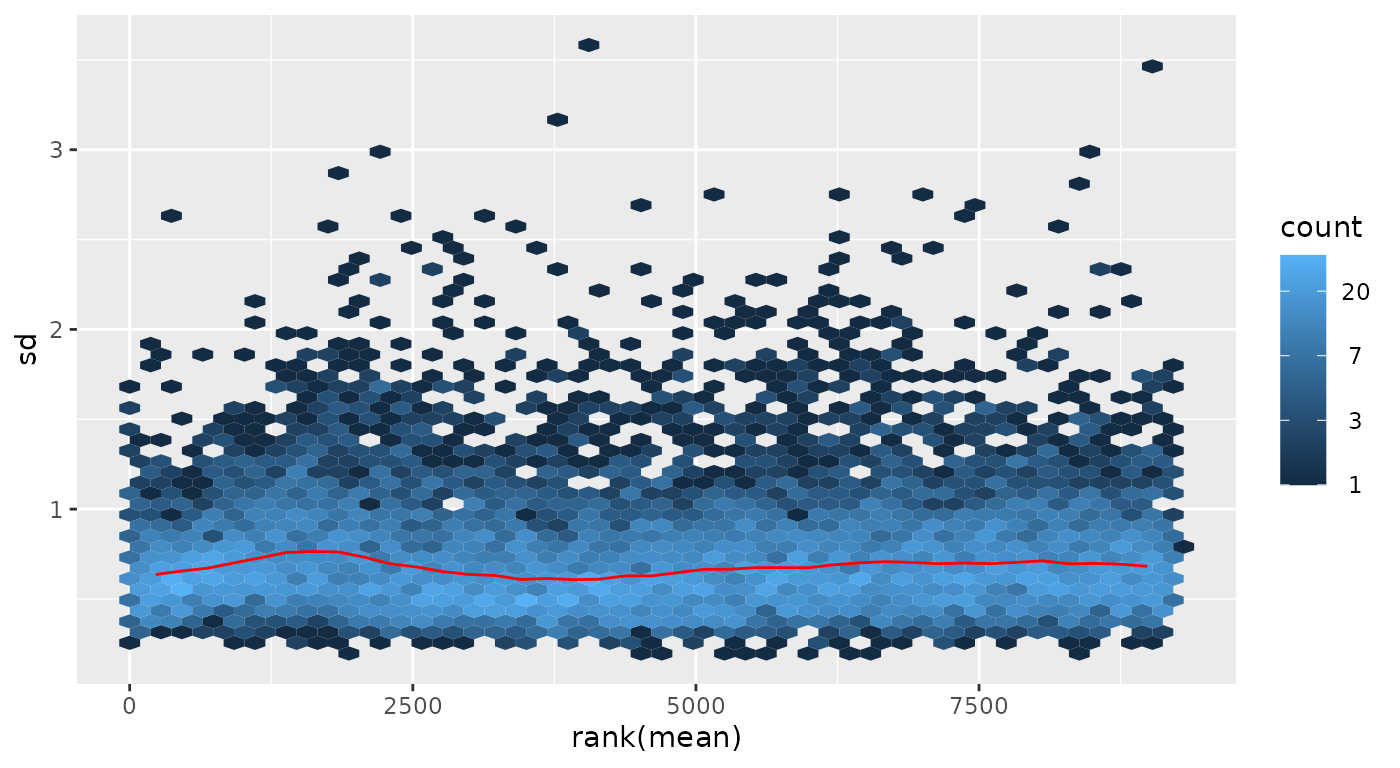

Standard deviation versus rank of the mean for the lymphoma example data

We see that the variance stabilisation worked. As above, we can obtain the generalised log-ratios for each slide by subtracting the common reference intensities from those for the 8 samples:

iref = seq(1, 15, by=2)
ismp = seq(2, 16, by=2)
M = exprs(lym)[,ismp]-exprs(lym)[,iref] 
A =(exprs(lym)[,ismp]+exprs(lym)[,iref])/2
colnames(M) = lymphoma$sample[ismp]
colnames(A) = colnames(M)

j = "DLCL-0032"
smoothScatter(A[,j], M[,j], main=j, xlab="A", ylab="M", pch=".")
abline(h=0, col="red")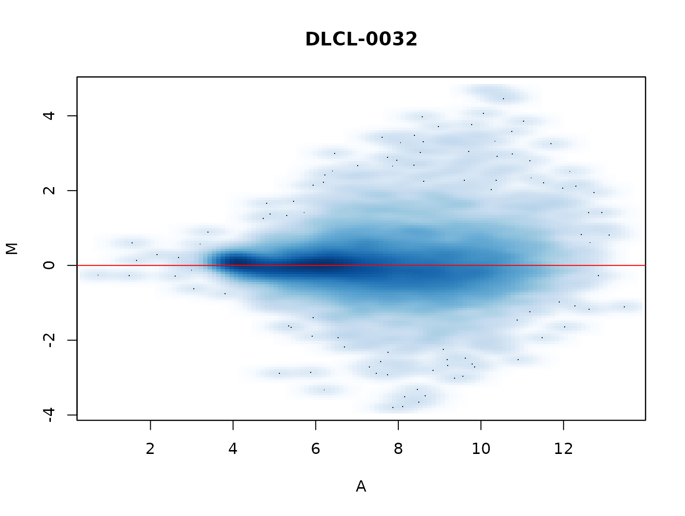

MA-plot for slide DLCL-0032 from the lymphoma example data. A false-colour representation of the data point density is used, in addition the 100 data points in the least dense regions are plotted as dots.

Running VSN on Affymetrix genechip data

The package affy provides excellent functionality for reading and processing Affymetrix genechip data, and you are encouraged to refer to the documentation of the package affy for more information about data structures and methodology. % The preprocessing of Affymetrix genechip data involves the following steps: (i) background correction, (ii) between-array normalization, (iii) transformation and (iv) summarisation. The VSN method addresses steps (i)–(iii). For the summarisation, I recommend to use the RMA method (Irizarry et al. 2003), and a simple wrapper that provides all of these is provided through the method vsnrma.

library("affydata")
data("Dilution")
d_vsn = vsnrma(Dilution)

For comparison, we also run rma.

d_rma = rma(Dilution)

par(mfrow = c(1, 3))
ax = c(2, 16)

plot(exprs(d_vsn)[,c(1,3)], main = "vsn: array 1 vs 3", asp = 1, xlim = ax, ylim = ax, pch = ".")

plot(exprs(d_rma)[,c(1,3)], main = "rma: array 1 vs 3", asp = 1, xlim = ax, ylim = ax, pch = ".")

plot(exprs(d_rma)[,1], exprs(d_vsn)[,1], 
     xlab = "rma", ylab = "vsn", asp = 1, xlim = ax, ylim = ax, main = "array 1", pch = ".")
abline(a = 0,  b =1, col = "#ff0000d0")

Results of vsnrma and rma on the Dilution data. Array 1 was hybridised with 20$\mu$g RNA from liver, Array 3 with 10$\mu$g of the same RNA.

Both methods control the variance at low intensities, but we see that VSN does so more strongly. See also Section @ref(sec:shrink) for further discussion on the VSN shrinkage.

Running VSN on RGList objects

There is a justvsn method for RGList objects. Usually, you will produce an RGList from your own data using the read.maimages from the limma package. Here, for the sake of demonstration, we construct an RGList from lymphoma.

library("limma")
wg = which(lymphoma$dye=="Cy3")
wr = which(lymphoma$dye=="Cy5")

lymRG = new("RGList", list(
  R=exprs(lymphoma)[, wr],
  G=exprs(lymphoma)[, wg]))

lymNCS = justvsn(lymRG)

The justvsn method for RGList converts its argument into an NChannelSet, using a copy of the coercion method from Martin Morgan in the package convert. It then passes this on to the justvsn method for NChannelSet. The return value is an NChannelSet, as shown below.

lymNCS

## NChannelSet (storageMode: lockedEnvironment)
## assayData: 9216 features, 8 samples 
##   element names: G, R 
## protocolData: none
## phenoData: none
## featureData: none
## experimentData: use 'experimentData(object)'
## Annotation:

Note that, due to the flexibility in the amount and quality of metadata that is in an RGList, and due to differences in the implementation of these classes, the transfer of the metadata into the NChannelSet may not always produce the expected results, and that some checking and often further dataset-specific postprocessing of the sample metadata and the array feature annotation is needed. For the current example, we construct the AnnotatedDataFrame object adf and assign it into the phenoData slot of lymNCS.

vmd = data.frame(
  labelDescription = I(c("array ID", "sample in G", "sample in R")),
  channel = c("_ALL", "G", "R"),
  row.names = c("arrayID", "sampG", "sampR"))

arrayID = lymphoma$name[wr]
stopifnot(identical(arrayID, lymphoma$name[wg])) 

## remove sample number suffix 
sampleType = factor(sub("-.*", "", lymphoma$sample)) 

v = data.frame(
  arrayID = arrayID,
  sampG   = sampleType[wg],
  sampR   = sampleType[wr])
v

##   arrayID     sampG sampR
## 1 lc7b047 reference   CLL
## 2 lc7b048 reference   CLL
## 3 lc7b069 reference   CLL
## 4 lc7b070 reference   CLL
## 5 lc7b019 reference  DLCL
## 6 lc7b056 reference  DLCL
## 7 lc7b057 reference  DLCL
## 8 lc7b058 reference  DLCL

adf = new("AnnotatedDataFrame", 
  data = v,
  varMetadata = vmd)

phenoData(lymNCS) = adf 

Now let us combine the red and green values from each array into the glog-ratio M and use the linear modeling tools from limma to find differentially expressed genes (note that it is often suboptimal to only consider M, and that taking into account absolute intensities as well can improve analyses).

lymM = (assayData(lymNCS)$R - 
        assayData(lymNCS)$G)

design = model.matrix( ~ lymNCS$sampR)
lf = lmFit(lymM, design[, 2, drop=FALSE])
lf = eBayes(lf)

The following plots show the resulting $p$-values and the expression profiles of the genes corresponding to the top 5 features.

par(mfrow=c(1,2))
hist(lf$p.value, breaks = 100, col="orange") 
pdat = t(lymM[order(lf$p.value)[1:5],])
matplot(pdat, lty = 1, type = "b", lwd = 2, col=hsv(seq(0,1,length=5), 0.7, 0.8), 
  ylab = "M", xlab = "arrays")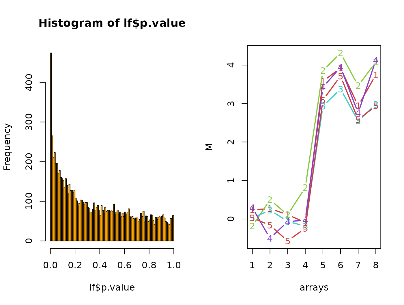

Left: histogram of p-values from the moderated $t$-test between the CLL and DLCL groups on the lymM values. Right: M-values for the 5 genes with the smallest p-values.

Background subtraction

Many image analysis programmes for microarrays provide local background estimates, which are typically calculated from the fluorescence signal outside, but next to the features. These are not always useful. Just as with any measurement, these local background estimates are also subject to random measurement error, and subtracting them from the foreground intensities will lead to increased random noise in the signal. On the other hand side, doing so may remove systematic artifactual drifts in the data, for example, a spatial gradient.

So what is the optimal analysis strategy, should you subtract local background estimates or not? The answer depends on the properties of your particular data. VSN itself estimates and subtracts an over-all background estimate (per array and colour, see Section @ref(sec:calib)), so an additional local background correction is only useful if there actually is local variability across an array, for example, a spatial gradient.

Supposing that you have decided to subtract the local background estimates, how is it done? When called with the argument backgroundsubtract=TRUE⁹, the justvsn method will subtract local background estimates in the Rb and Gb slots of the incoming RGList. To demonstrate this, we construct an RGList object lymRGwbg.

rndbg = function(x, off, fac)
   array(off + fac * runif(prod(dim(x))), dim = dim(x))

lymRGwbg    = lymRG
lymRGwbg$Rb = rndbg(lymRG, 100, 30)
lymRGwbg$Gb = rndbg(lymRG,  50, 20)

In practice, of course, these values will be read from the image quantitation file with a function such as read.maimages that produces the RGList object. We can call justvsn

lymESwbg = justvsn(lymRGwbg[, 1:3], backgroundsubtract=TRUE)

Here we only do this for the first 3 arrays to save compute time.

Print-tip groups

By default, VSN computes one normalisation transformation with a common set of parameters for all features of an array (separately for each colour if it is a multi-colour microarray), see Section @ref(sec:calib). Sometimes, there is a need for stratification by further variables of the array manufacturing process, for example, print-tip groups (sectors) or microtitre plates. This can be done with the strata parameter of vsn2.

The example data that comes with the package does not directly provide the information which print-tip each feature was spotted with, but we can easily reconstruct it:

ngr = ngc = 4L
nsr = nsc = 24L
arrayGeometry = data.frame(
  spotcol = rep(1:nsc, times = nsr*ngr*ngc),
  spotrow = rep(1:nsr, each = nsc, times=ngr*ngc),
  pin = rep(1:(ngr*ngc), each = nsr*nsc))

and call

EconStr = justvsn(lymRG[, 1], strata = arrayGeometry$pin)

To save CPU time, we only call this on the first array. We compare the result to calling justvsn without strata,

EsenzaStr = justvsn(lymRG[, 1])

A scatterplot comparing the transformed red intensities, using the two models, is shown in Figure @ref(fig:figstrata2).

j = 1
plot(assayData(EsenzaStr)$R[,j],
     assayData(EconStr)$R[,j],
     pch = ".", asp = 1, 
     col = hsv(seq(0, 1, length=ngr*ngc), 
       0.8, 0.6)[arrayGeometry$pin], 
     xlab = "without strata", 
     ylab = "print-tip strata",
     main = sampleNames(lymNCS)$R[j])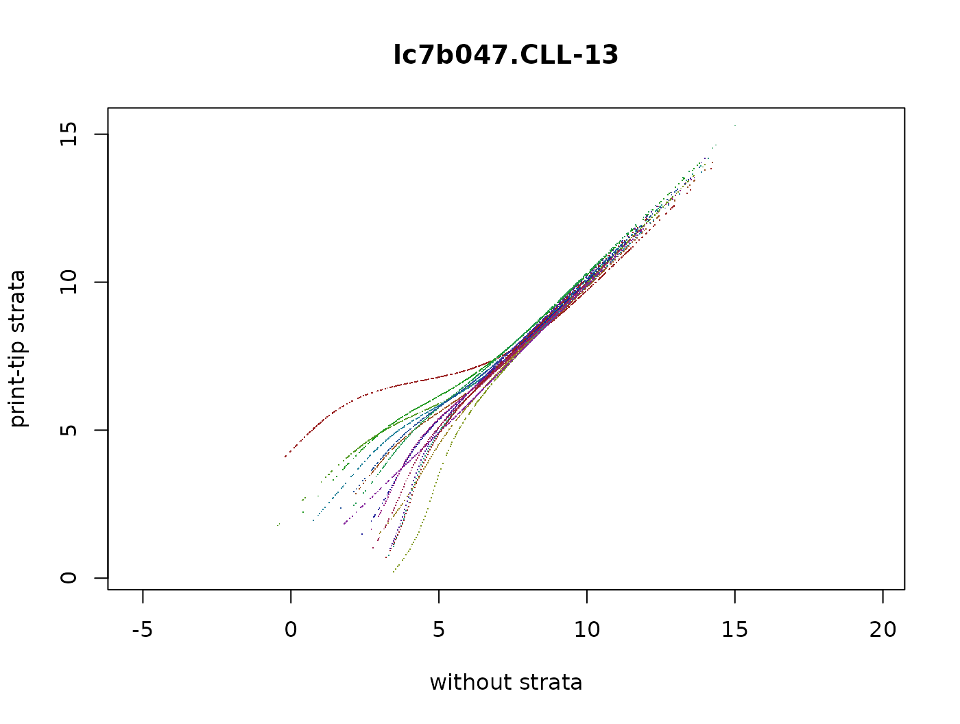

Scatterplot of normalised and transformed intensities for the red channel of Array 1. Values on the $x$-axis correspond to normalisation without strata (EsenzaStr), values on the $y$-axis to normalisation with strata (EconStr). The different colours correspond to the 16 different strata.

Missing values

The parameter estimation algorithm of VSN is able to deal with missing values in the input data. To demonstrate this, we generate an ExpressionSet lym2 in which about 10% of all intensities are randomly missing,

lym2 = lymphoma
nfeat = prod(dim(lym2))
wh = sample(nfeat, nfeat/10)
exprs(lym2)[wh] = NA
table(is.na(exprs(lym2)))

## 
##  FALSE   TRUE 
## 132711  14745

and call vsn2 on it.

fit1 = vsn2(lymphoma, lts.quantile=1)
fit2 = vsn2(lym2, lts.quantile=1)

The resulting fitted parameters are not identical, but very similar, see Figure @ref(fig:miss). %

par(mfrow=c(1,2))
for(j in 1:2){
  p1 = coef(fit1)[,,j]
  p2 = coef(fit2)[,,j]
  d  = max(abs(p1-p2))
  stopifnot(d < c(0.05, 0.03)[j])
  plot(p1, p2, pch = 16, asp = 1,
    main = paste(letters[j], 
      ": max diff=", signif(d,2), sep = ""),
    xlab = "no missing data",
    ylab = "10% of data missing")
  abline(a = 0, b = 1, col = "blue")
}

Scatterplots of fitted parameters, values on the $x$-axis correspond to normalisation without missing data (fit1), values on the $y$-axis to normalisation with around 10% missing data (fit2).

Note that p1 and p2 would differ more if we used a different value than 1 for the lts.quantile argument in the above calls of vsn2. This is because the outlier removal algorithm will, for this dataset, identify different sets of features as outliers for fit1 and fit2 and consequently the optimisation result will be slightly different; this difference is arguably negligible compared to the noise level in the data.

Normalisation with ‘spike-in’ probes

Normally, VSN uses all features on the array to fit the calibration and transformation parameters, and the algorithm relies, to a certain extent, on the assumption that most of the features’ target genes are not differentially expressed (see also Section @ref(sec:mostunch)). If certain features are known to correspond to, or not to correspond to, differentially expressed targets, then we can help the algorithm by fitting the calibration and transformation parameters only to the subset of features for which the “not differentially expressed” assumption is most appropriate, and then applying the calibration and transformation to all features. For example, some experimental designs provide “spike-in” control spots for which we know that their targets’ abundance is the same across all arrays (and/or colours).

For demonstration, let us assume that in the kidney data, features 100 to 200 are spike-in controls. Then we can obtain a normalised dataset nkid as follows.

spikeins = 100:200
spfit = vsn2(kidney[spikeins,], lts.quantile=1)
nkid = predict(spfit, newdata=kidney)

Note that if we are sufficiently confident that the spikeins subset is really not differentially expressed, and also has no outliers for other, say technical, reasons, then we can set the robustness parameter lts.quantile to 1. This corresponds no robustness (least sum of squares regression), but makes most use of the data, and the resulting estimates will be more precise, which may be particularly important if the size of the spikeins set is relatively small.

Not that this explicit subsetting strategy is designed for features for which we have a priori knowledge that their normalised intensities should be unchanged. There is no need for you to devise data-driven rules such as using a first call to VSN to get a preliminary normalisation, identify the least changing features, and then call VSN again on that subset. This strategy is already built into the VSN algorithm and is controlled by its lts.quantile parameter. Please see Section @ref(sec:mostunch) and reference (Huber, Heydebreck, Sültmann, et al. 2003) for details.

Normalisation against an existing reference dataset

So far, we have considered the joint normalisation of a set of arrays to each other. What happens if, after analysing a set of arrays in this fashion, we obtain some additonal arrays? Do we re-run the whole normalisation again for the complete, new and bigger set of arrays? This may sometimes be impractical.

Suppose we have used a set of training arrays for setting up a classifier that is able to discriminate different biological states of the samples based on their mRNA profile. Now we get new test arrays to which we want to apply the classifier. Clearly, we do not want to re-run the normalisation for the whole, new and bigger dataset, as this would change the training data; neither can we normalise only the test arrays among themselves, without normalising them towards the reference training dataset. What we need is a normalisation procedure that normalises the new test arrays towards the existing reference dataset without changing the latter.

To simulate this situation with the available example data, pretend that the Cy5 channels of the lymphoma dataset can be treated as 8 single-colour arrays, and fit a model to the first 7.

ref = vsn2(lymphoma[, ismp[1:7]])

Now we call vsn2 on the 8-th array, with the output from the previous call as the reference.

f8 = vsn2(lymphoma[, ismp[8]], reference = ref)

We can compare this to what we get if we fit the model to all 8 arrays,

fall = vsn2(lymphoma[, ismp])

coefficients(f8)[,1,]

## [1] -0.396 -3.509

coefficients(fall)[,8,]

## [1] -0.323 -3.507

and compare the resulting values in the scatterplot shown in Figure @ref(fig:ref): they are very similar.

plot(exprs(f8), exprs(fall)[,8], pch = ".", asp = 1)
abline(a = 0, b = 1, col = "red")

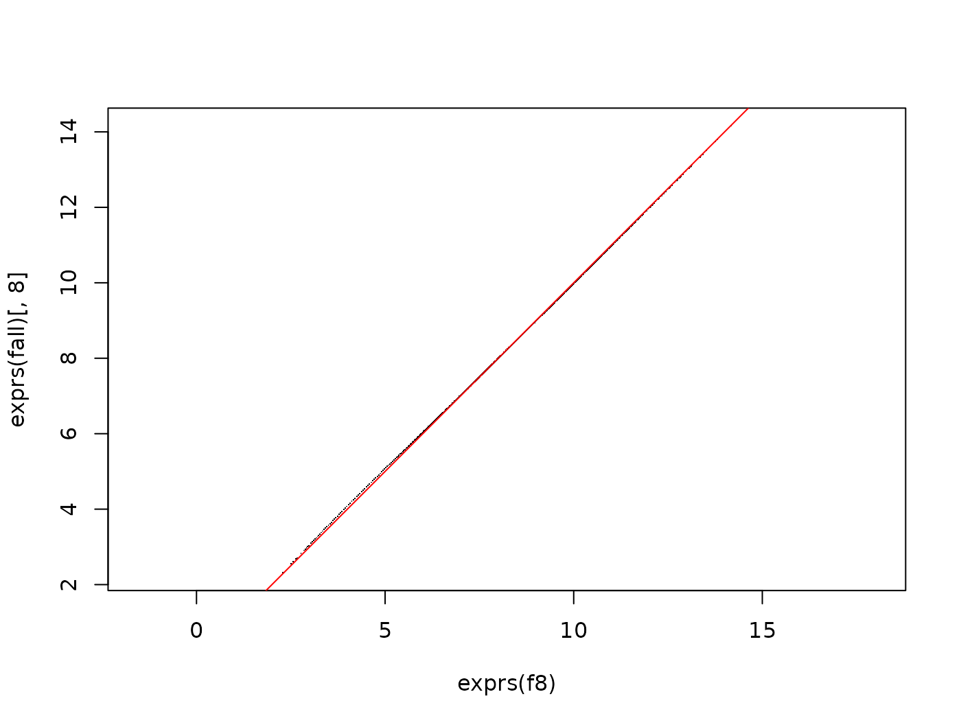
Scatterplot of normalised intensities after normalisation by reference ($x$-axis, f8) and joint normalisation ($y$-axis, fall). There is good agreement.

More details on this can be found in the vignettes Verifying and assessing the performance with simulated data and Likelihood Calculations for vsn that come with this package.

The calibration parameters

If $y_{ki}$ is the matrix of uncalibrated data, with $k$ indexing the rows and $i$ the columns, then the calibrated data $y_{ki}'$ is obtained through scaling by $\lambda_{si}$ and shifting by $\alpha_{si}$:

$$\begin{equation} y_{ki}' = \lambda_{si}y_{ki}+\alpha_{si} (\#eq:cal) \end{equation}$$

where $s\equiv s(k)$ is the so-called stratum for feature $k$. In the simplest case, there is only one stratum, i.e. the index $s$ is always equal to 1, or may be omitted altogether. This amounts to assuming that the data of all features on an array were subject to the same systematic effects, such that an array-wide calibration is sufficient.

A model with multiple strata per array may be useful for spotted arrays. For these, stratification may be according to print-tip (Dudoit et al. 2002) or PCR-plate (Huber, Heydebreck, and Vingron 2003). For oligonucleotide arrays, it may be useful to stratify the features by physico-chemical properties, e.g., to assume that features of different sequence composition attract systematically different levels of unspecific background signal.

The transformation to a scale where the variance of the data is approximately independent of the mean is

$$\begin{eqnarray} h_{ki} &=& \text{arsinh}(\lambda_0y_{ki}'+\alpha_0) (\#eq:vs) \\ &=& \log\left( \lambda_0y_{ki}'+\alpha_0+ \sqrt{\left(\lambda_0y_{ki}'+\alpha_0\right)^2+1}\right),\nonumber \end{eqnarray}$$

with two parameters $\lambda_0$ and $\alpha_0$. Equations @ref(eq:cal) and @ref(eq:vs) can be combined, so that the whole transformation is given by

$$\begin{equation} h_{ki} = \text{arsinh}\left(e^{b_{si}}\cdot y_{ki}+a_{si}\right). (\#eq:transf) \end{equation}$$

Here, $a_{si}=\alpha_{si}+\lambda_0\alpha_{si}$ and $b_{si}=\log(\lambda_0\lambda_{si})$ are the combined calibation and transformation parameters for features from stratum $s$ and sample $i$. Using the parameter $b_{si}$ as defined here rather than $e^{b_{si}}$ appears to make the numerical optimisation more reliable (less ill-conditioned).

We can access the calibration and transformation parameters through

coef(fit)[1,,]

##        [,1]  [,2]
## [1,] -0.550 -5.84
## [2,] -0.535 -5.86

For a dataset with $d$ samples and $s$ strata, coef(fit) is a numeric array with dimensions $(s, d, 2)$. For the example data that was used in Section @ref(sec:overv) to generate fit, $d=2$ and $s=1$. coef(fit)[s, i, 1], the first line in the results of the above code chunk, is what was called $a_{si}$ in Eqn. @ref(eq:transf), and coef(fit)[s, i, 2], the second line, is $b_{si}$.

The calibration parameters and the additive-multiplicative error model

VSN is based on the additive-multiplicative error model Huber et al. (2004), which predicts a quadratic variance-mean relationship of the form (Huber et al. 2002)

$$\begin{equation} v(u)=(c_1u+c_2)^2+c_3. \end{equation}$$

This is a general parameterization of a parabola with three parameters $c_1$, $c_2$ and $c_3$. Here, $u$ is the expectation value (mean) of the signal, and $v$ the variance. $c_1$ is also called the coefficient of variation, since for large $u$, $\sqrt{v}/u\approx c_1$. The minimum of $v$ is $c_3$, this is the variance of the additive noise component. It is attained at $u=-c_2/c_3$, and this is the expectation value of the additive noise component, which ideally were zero ($c_2=0$), but in many applications is different from zero. Only the behaviour of $v(u)$ for $u\ge -c_2/c_3$ is typically relevant.

The parameters $a$ and $b$ from Equation @ref(eq:transf)¹⁰ and the parameters of the additive-multiplicative error model are related by (Huber et al. 2002)

$$\begin{eqnarray} a&=&\frac{c_2}{\sqrt{c_3}}\nonumber\\ e^b&=&\frac{c_1}{\sqrt{c_3}}(\#eq:errmod2trsf) \end{eqnarray}$$

This relationship is not 1:1, and it has a divergence at $c_3\to0$; both of these observations have practical consequences, as explained in the following.

1. The fact that Equations @ref(eq:errmod2trsf) do not constitute a 1:1 relationship means that multiple parameter sets of the additive-multiplicative error model can lead to the same transformation. This can be resolved, for example, if the coefficient of variation $c_1$ is obtained by some other means than the vsn2 function. For example, it can be estimated from the standard deviation of the VSN-transformed data, which is, in the approximation of the delta method, the same as the coefficient of variation Huber, Heydebreck, Sültmann, et al. (2003). Then,

$$\begin{eqnarray} c_3&=& c_1^2\, e^{-2b}\nonumber\\ c_2&=& c_1 \, a e^{-b}.(\#eq:trsf2errmod) \end{eqnarray}$$

2. The divergence for $c_3\to0$ can be a more serious problem. In some datasets, $c_3$ is in fact very small. This is the case if the size of the additive noise is negligible compared to the multiplicative noise throughout the dynamic range of the data, even for the smallest intensities. In other words, the additive-multiplicative error model is overparameterized, and a simpler multiplicative-only model would be good enough. VSN is designed to still produce reasonable results in these cases, in the sense that the transformation stabilizes the variance (it turns essentially into the usual logarithm transformation), but the resulting fit coefficients can be unstable.

The assessment of the precision of the estimated values of $a$ and $b$ (e.g. by resampling, or by using replicate data) is therefore usually not very relevant; what is relevant is an assessment of the precision of the estimated transformation, i.e. how much do the transformed values vary (Huber, Heydebreck, Sültmann, et al. 2003).

More on calibration

Now suppose the kidney example data were not that well measured, and the red channel had a baseline that was shifted by 500 and a scale that differed by a factor of $0.25$:

bkid = kidney
exprs(bkid)[,1] = 0.25*(500+exprs(bkid)[,1])

We can again call vsn2 on these data

bfit = vsn2(bkid)

plot(exprs(bkid), main = "raw", pch = ".", log = "xy")

Scatterplot for the badly biased bkid data: log-log scale.

plot(exprs(bfit), main = "vsn", pch = ".")

Scatterplot for the badly biased bkid data: after calibration and transformation with vsn.

coef(bfit)[1,,]

##        [,1]  [,2]
## [1,] -2.011 -4.45
## [2,] -0.535 -5.86

Notice the change in the parameter $b$ of the red channel: it is now larger by about $\log(4)\approx 1.4$, and the shift parameter $a$ has also been adjusted.

Variance stabilisation without calibration

It is possible to force $\lambda_{si}=1$ and $\alpha_{si}=0$ for all $s$ and $i$ in Equation @ref(eq:cal) by setting vsn2’s parameter calib to none. Hence, only the global variance stabilisation transformation @ref(eq:vs) will be applied, but no column- or row-specific calibration.

Here, I show an example where this feature is used in conjunction with quantile normalisation.

lym_q = normalizeQuantiles(exprs(lymphoma))
lym_qvsn = vsn2(lym_q, calib="none")
plot(exprs(lym_qvsn)[, 1:2], pch=".", main="lym_qvsn")

Scatterplot between the red and green intensities of the array of the lymphoma dataset after quantile normalisation followed by VSN variance stabilisation without calibration.

plot(exprs(lym)[,1], exprs(lym_qvsn)[, 1], 
  main="lym_qvsn vs lym", pch=".", 
  ylab="lym_qvsn[,1]", xlab="lym[,1]")

Comparison of the values calculated in this section, for CH1 of the first array, to those of VSN variance stabilisation with affine calibration (lym was computed in Section @ref(sec:lymphoma)).

Assessing the performance of VSN

VSN is a parameter estimation algorithm that fits the parameters for a certain model. In order to see how good the estimator is, we can look at bias, variance, sample size dependence, robustness against model misspecificaton and outliers. This is done in the vignette Verifying and assessing the performance with simulated data that comes with this package.

Practically, the more interesting question is how different microarray calibration and data transformation methods compare to each other. Two such comparisons were made in reference (Huber et al. 2002), one with a set of two-colour cDNA arrays, one with an Affymetrix genechip dataset. Fold-change estimates from VSN led to higher sensitivity and specificity in identifying differentially expressed genes than a number of other methods.

A much more sophisticated and wider-scoped approach was taken by the Affycomp benchmark study. It uses two benchmark datasets: a Spike-In dataset, in which a small number of cDNAs was spiked in at known concentrations and over a wide range of concentrations on top of a complex RNA background sample; and a Dilution dataset, in which RNA samples from heart and brain were combined in a number of dilutions and proportions. The design of the benchmark study, which has been open for anyone to submit their method, was described in (Cope et al. 2004). A discussion of its results was given in (Irizarry et al. 2006). One of the results that emerged was that VSN compares well with the background correction and quantile normalization method of RMA; both methods place a high emphasis on precision of the expression estimate, at the price of a certain bias (see also Section @ref(sec:shrink)). Another result was that reporter-sequence specific effects (e.g., the effect of GC content) play a large role in these data and that substantial improvements can be achieved when they are taken into account (something which VSN does not do).

Of course, the two datasets that were used in Affycomp were somewhat artificial: they had fewer differentially expressed genes and were probably of higher quality than in most real-life applications. And, naturally, in the meanwhile the existence of this benchmark has led to the development of new processing methods where a certain amount of overfitting may have occured.

I would also like to note the interaction between normalization/preprocessing and data quality. For data of high quality, one can argue that any decent preprocessing method should produce more or less the same results; differences arise when the data are problematic, and when more or less successful measures may be taken by preprocessing methods to correct these problems.

VSN, shrinkage and background correction

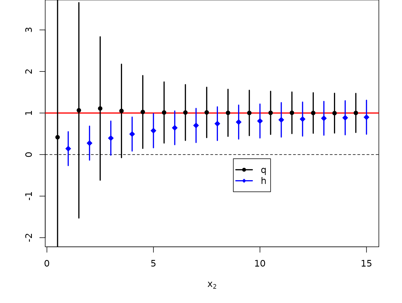
The shrinkage property of the generalised log-ratio. Blue diamonds and error bars correspond to mean and standard deviation of the generalised log-ratio $h$, as obtained from VSN, and black dots and error bars to the standard log-ratio $q$ (both base 2).

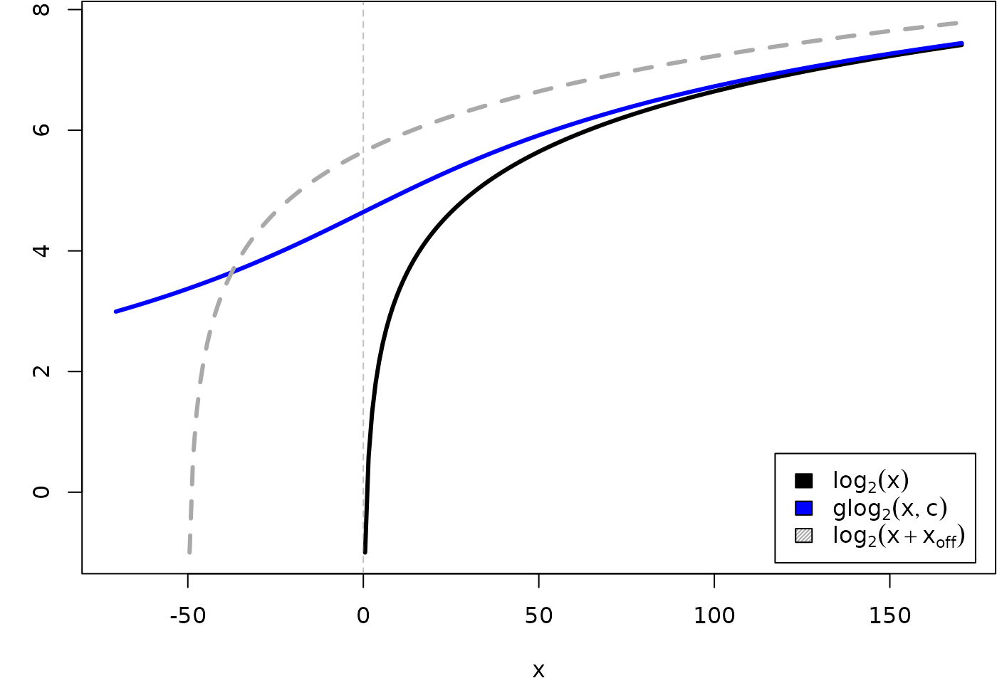
Graphs of the functions. $y=\log_2(x)$, $y=$glog$_2(x,c)=\log_2(x+\sqrt{x^2+c^2})-1$, and $y=\log_2(x+x_{\text{off}})$, where $c=50$ and $x_{\text{off}}=50$.

Generalised log-ratios can be viewed as a shrinkage estimator: for low intensities either in the numerator and denominator, they are smaller in absolute value than the standard log-ratios, whereas for large intensities, they become equal. Their advantage is that they do not suffer from the variance divergence of the standard log-ratios at small intensities: they remain well-defined and have limited variance when the data come close to zero or even become negative.

An illustration is shown in Figure @ref(fig:shrink). Data were generated from the additive-multiplicative error model Huber et al. (2004). The horizontal line corresponds to the true $\log_2$-ratio $1$ (corresponding to a factor of 2). For intensities $x_2$ that are larger than about ten times the additive noise level $\sigma_a$, generalised log-ratio $h$ and standard log-ratio $q$ coincide. For smaller intensities, we can see a variance-bias trade-off: $q$ has almost no bias, but a huge variance, thus an estimate of the fold change based on a limited set of data can be arbitrarily off. In contrast, $h$ keeps a constant variance – at the price of systematically underestimating the true fold change. This is the main argument for using a variance stabilising transformation.

Note that there is also some bias in the behaviour of $q$ for small $x_2$, particularly at $x_2=0.5$. This results from the occurence of negative values in the data, which are discarded from the sampling when the (log-)ratio is computed.

Please consult the references for more on the mathematical background Huber, Heydebreck, Sültmann, et al. (2003).

It is possible to give a Bayesian interpretation: our prior assumption is the conservative one of no differential expression. Evidence from a feature with high overall intensity is taken strongly, and the posterior results in an estimate close to the empirical intensity ratio. Evidence from features with low intensity is downweighted, and the posterior is still strongly influenced by the prior.

Quality assessment

Quality problems can often be associated with physical parameters of the manufacturing or experimental process. Let us look a bit closer at the lymphoma data. Recall that M is the 9216 times 8 matrix of generalized log-ratios and A a matrix of the same size with the average glog$_2$-transformed intensities. The dataframe arrayGeometry (from Section @ref(sec:strata)) contains, for each array feature, the identifier of the print-tip by which it was spotted and the row and column within the print-tip sector. Figure @ref(fig:lymbox) shows the boxplots of A values of array CLL-13 stratified by row.

colours = hsv(seq(0,1, length = nsr), 0.6, 1)
j = "CLL-13"
boxplot(A[, j] ~ arrayGeometry$spotrow, col = colours, main = j, ylab = "A", xlab = "spotrow")

Boxplot of A values of array CLL-13 stratified by within-sector row. The features in rows 22 and 23 are all very dim.

You may want to explore similar boxplots for other stratifying factors such as column within print-tip sector or print-tip sector and look at these plots for the other arrays as well.

In Figure @ref(fig:lymbox), we see that the features in rows 22 and 23 are all very dim. If we now look at these data in the $M$-$A$-plot (Figure @(fig:lymquscp)), we see that these features not only have low $A$-values, but fall systematically away from the $M=0$ line.

plot(A[,j], M[,j], pch = 16, cex = 0.3,
  col = ifelse(arrayGeometry$spotrow%in%(22:23), "orange", "black"))
abline(h = 0, col = "blue")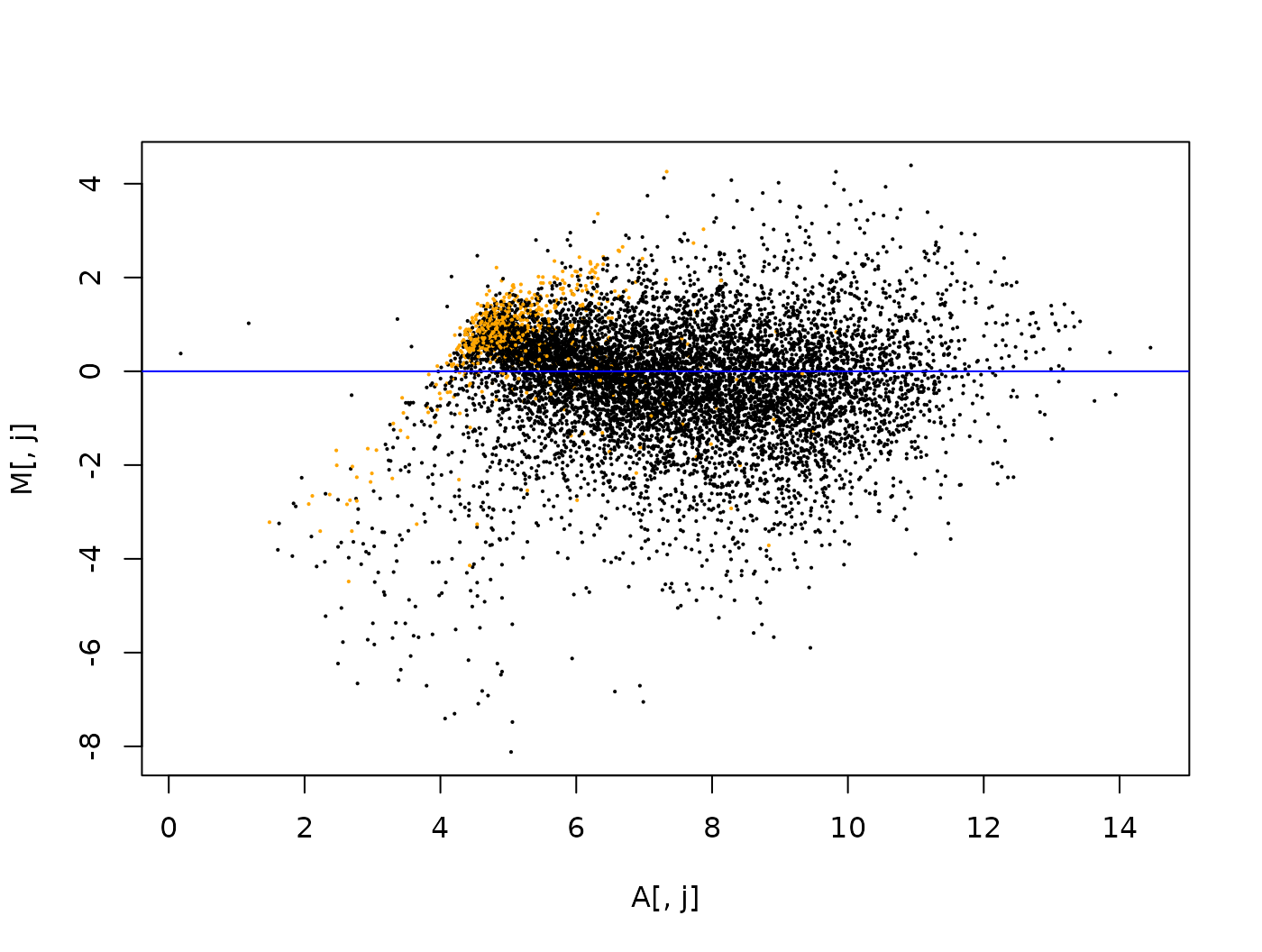

MA-plot of the data from array r j. Dots coloured in orange are from rows 22 and 23. A possible explanation may be as follows (although I do not know for sure that this is the right explanation): The PCR product (cDNA) that is spotted on these arrays is put on by a print head that sucks cDNA out of microtitre plates and deposits them in spots one after another, row by row. If the content of one plate is faulty, this results in a set of subsequent spots that are faulty. Because the 16 print-tip sectors are spotted in parallel, this affects all sectors in the same way.

Hence, in a naive analysis the data from these features would be interpreted as contributing evidence for differential expression, while they are more likely just the result of a quality problem. So what can we do? There are some options:

• Flag the data of the affected features as unreliable and set them aside from the subsequent analysis.
• Use a more complex, stratified normalisation method that takes into account the different row behaviours, for example, VSN with strata (see Section @ref(sec:strata)).
• It has also been proposed to address this type of problem by using a non-linear regression on the $A$-values, for example the loess normalization of reference (Yang et al. 2001) that simply squeezes the $M$-$A$-plot to force the centre of the distribution of $M$ to lie at 0 along the whole $A$-range.

An advantage of Option 3 is that it works without knowing the real underlying stratifying factor. However, it assumes that the stratifying factor is strongly confounded with $A$, and that biases that it causes can be removed through a regression on $A$.

In the current example, if we believe that the real underlying stratifying factor is indeed row within sector, this assumption means that (i) few of the data points from rows 22 and 23 have high $A$-values, and that (ii) almost all data points with very low $A$ values are from these rows; while (i) appears tenable, (ii) is definitely not the case.

Stratifying factors such as print-tip, PCR plate, reporter-sequence

By default, the VSN method assumes that the measured signal $y_{ik}$ increases, to sufficient approximation, proportionally to the mRNA abundance $c_{ik}$ of gene $k$ on array $i$ (or in colour channel $i$):

$$\begin{equation} y_{ik}\approx \alpha_i + \lambda_i \lambda_k c_{ik}. (\#eq:assumption1) \end{equation}$$

For a series of $d$ single-colour arrays, $i=1,\ldots,d$, and the different factors $\lambda_i$ reflect the different initial amounts of sample mRNA or different overall reverse transcription, hybridisation and detection efficiencies. The feature affinity $\lambda_k$ contains factors that affect all measurements with feature $k$ in the same manner, such as sequence-specific labelling efficiency. The $\lambda_k$ are assumed to be the same across all arrays. There can be a non-zero overall offset $\alpha_i$. For a two-colour cDNA array, $i=1,2$, and the $\lambda_i$ take into account the different overall efficiencies of the two dyes¹¹.

Equation @ref(eq:assumption1) can be generalised to

$$\begin{equation} y_{ik}\approx \alpha_{is} + \lambda_{is} \lambda_k c_{ik}. (\#eq:assumption2) \end{equation}$$

that is, the background term $\alpha_{is}$ and the gain factor $\lambda_{is}$ can be different for different groups $s$ of features on an array. The VSN methods allows for this option by using the strata argument of the function vsn2. We have seen an example above where this could be useful. For Affymetrix genechips, one can find systematic dependences of the affinities $\lambda_{is}$ and the background terms $\alpha_{is}$ on the reporter sequence.

Nevertheless, there are situations in which either assumption @ref(eq:assumption1) or @ref(eq:assumption2) is violated, and these include:

Saturation

The biochemical reactions and/or the photodetection can be run in such a manner that saturation effects occur. It may be possible to rescue such data by using non-linear transformations. Alternatively, it is recommended that the experimental parameters are chosen to avoid saturation.

Batch effects

The feature affinities $\lambda_k$ may differ between different manufacturing batches of arrays due, e.g., to different qualities of DNA amplification or printing. VSN cannot be used to simultaneously calibrate and transform data from different batches.

How to reliably diagnose and deal with such violations is beyond the scope of this vignette; see the references for more Dudoit et al. (2002).

Most genes unchanged assumption

With respect to the VSN model fitting, data from differentially transcribed genes can act as outliers (but they do not necessarily need to do so in all cases). The maximal number of outliers that do not gravely affect the model fitting is controlled by the parameter lts.quantile. Its default value is 0.9, which allows for 10% outliers. The value of lts.quantile can be reduced down to 0.5, which allows for up to 50% outliers. The maximal value is 1, which results in a least-sum-of-squares estimation that does not allow for any outliers.

So why is this parameter lts.quantile user-definable and why don’t we just always use the most “robust” value of 0.5? The answer is that the precision of the estimated VSN parameters is better the more data points go into the estimates, and this may especially be an issue for arrays with a small number of features¹². So if you are confident that the number of outliers is not that large, using a high value of lts.quantile can be justified.

There has been confusion on the role of the ``most genes unchanged assumption’’, which presumes that only a minority of genes on the arrays is detectably differentially transcribed across the experiments. This assumption is a sufficient condition for there being only a small number of outliers, and these would not gravely affect the VSN model parameter estimation. However, it is not a necessary condition: the parameter estimates and the resulting normalised data may still be useful if the assumption does not hold, but if the effects of the data from differentially transcribed genes balance out.

Acknowledgements

I acknowledge helpful comments and feedback from Anja von Heydebreck, Richard Bourgon, Martin Vingron, Ulrich Mansmann and Robert Gentleman. The active development of the vsn package was from 2001 to 2003, and most of this document was written during that time (although the current layout is more recent).

Session info

sessionInfo()

## R version 4.6.1 (2026-06-24)
## Platform: x86_64-pc-linux-gnu
## Running under: Ubuntu 24.04.5 LTS
## 
## Matrix products: default
## BLAS:   /usr/lib/x86_64-linux-gnu/openblas-pthread/libblas.so.3 
## LAPACK: /usr/lib/x86_64-linux-gnu/openblas-pthread/libopenblasp-r0.3.26.so;  LAPACK version 3.12.0
## 
## locale:
##  [1] LC_CTYPE=C.UTF-8       LC_NUMERIC=C           LC_TIME=C.UTF-8       
##  [4] LC_COLLATE=C.UTF-8     LC_MONETARY=C.UTF-8    LC_MESSAGES=C.UTF-8   
##  [7] LC_PAPER=C.UTF-8       LC_NAME=C              LC_ADDRESS=C          
## [10] LC_TELEPHONE=C         LC_MEASUREMENT=C.UTF-8 LC_IDENTIFICATION=C   
## 
## time zone: UTC
## tzcode source: system (glibc)
## 
## attached base packages:
## [1] stats     graphics  grDevices utils     datasets  methods   base     
## 
## other attached packages:
##  [1] limma_3.68.5        hgu95av2cdf_2.18.0  affydata_1.60.0    
##  [4] affy_1.90.0         ggplot2_4.0.3       vsn_3.81.1         
##  [7] Biobase_2.72.0      BiocGenerics_0.58.1 generics_0.1.4     
## [10] BiocStyle_2.40.0   
## 
## loaded via a namespace (and not attached):
##  [1] KEGGREST_1.52.2       gtable_0.3.6          xfun_0.61            
##  [4] bslib_0.12.0          lattice_0.22-9        vctrs_0.7.3          
##  [7] tools_4.6.1           stats4_4.6.1          tibble_3.3.1         
## [10] AnnotationDbi_1.74.0  RSQLite_3.53.3        blob_1.3.0           
## [13] pkgconfig_2.0.3       KernSmooth_2.23-26    RColorBrewer_1.1-3   
## [16] S7_0.2.2              desc_1.4.3            S4Vectors_0.50.3     
## [19] lifecycle_1.0.5       compiler_4.6.1        farver_2.1.2         
## [22] textshaping_1.0.5     Biostrings_2.80.2     statmod_1.5.2        
## [25] Seqinfo_1.2.0         codetools_0.2-20      htmltools_0.5.9      
## [28] sass_0.4.10           yaml_2.3.12           preprocessCore_1.74.0
## [31] crayon_1.5.3          hexbin_1.28.6         pillar_1.11.1        
## [34] pkgdown_2.2.1         jquerylib_0.1.4       cachem_1.1.0         
## [37] tidyselect_1.2.1      digest_0.6.39         dplyr_1.2.1          
## [40] bookdown_0.48         labeling_0.4.3        fastmap_1.2.0        
## [43] grid_4.6.1            cli_3.6.6             magrittr_2.0.5       
## [46] withr_3.0.3           scales_1.4.0          bit64_4.8.6          
## [49] XVector_0.52.0        rmarkdown_2.32        httr_1.4.9           
## [52] affyio_1.82.0         bit_4.6.0             otel_0.2.0           
## [55] ragg_1.5.2            png_0.1-9             memoise_2.0.1        
## [58] evaluate_1.0.5        knitr_1.52            IRanges_2.46.0       
## [61] rlang_1.3.0           glue_1.8.1            DBI_1.3.0            
## [64] BiocManager_1.30.27   jsonlite_2.0.0        R6_2.6.1             
## [67] systemfonts_1.3.2     fs_2.1.0

References

Alizadeh, Ash A., Michael B. Eisen, R. Eric Davis, et al. 2000. “Distinct Types of Diffuse Large B-Cell Lymphoma Identified by Gene Expression Profiling.” Nature 403: 503–11.

Cope, L. M., R. A. Irizarry, H. A. Jaffee, Z. Wu, and T. P. Speed. 2004. “A benchmark for Affymetrix GeneChip expression measures.” Bioinformatics 20 (3): 323–31.

Dudoit, Sandrine, Yee Hwa Yang, Terence P. Speed, and Matthew J. Callow. 2002. “Statistical Methods for Identifying Differentially Expressed Genes in Replicated cDNA Microarray Experiments.” Statistica Sinica 12: 111–39.

Huber, Wolfgang, Anja von Heydebreck, Holger Sültmann, Annemarie Poustka, and Martin Vingron. 2002. “Variance Stabilization Applied to Microarray Data Calibration and to the Quantification of Differential Expression.” Bioinformatics 18 Suppl 1: 96–104. http://bioinformatics.oxfordjournals.org/content/18/suppl_1/S96.abstract.

Huber, Wolfgang, Anja von Heydebreck, Holger Sültmann, Annemarie Poustka, and Martin Vingron. 2003. “Parameter Estimation for the Calibration and Variance Stabilization of Microarray Data.” Statistical Applications in Genetics and Molecular Biology 2 (1): Article 3. http://www.degruyter.com/view/j/sagmb.2003.2.1/sagmb.2003.2.1.1008/sagmb.2003.2.1.1008.xml.

Huber, Wolfgang, Anja von Heydebreck, and Martin Vingron. 2003. “Analysis of Microarray Gene Expression Data.” In Handbook of Statistical Genetics. John Wiley & Sons, Ltd.

Huber, Wolfgang, Anja von Heydebreck, and Martin Vingron. 2004. “Error Models for Microarray Intensities.” In Encyclopedia of Genetics, Genomics, Proteomics and Bioinformatics. John Wiley & Sons.

Irizarry, R. A., Z. Wu, and H. A. Jaffee. 2006. “Comparison of Affymetrix GeneChip expression measures.” Bioinformatics 22 (7): 789–94.

Irizarry, Rafael A., Bridget Hobbs, Francois Collin, et al. 2003. “Exploration, Normalization, and Summaries of High Density Oligonucleotide Array Probe Level Data.” Biostatistics 4: 249–64.

Rocke, David M., and Blythe Durbin. 2001. “A Model for Measurement Error for Gene Expression Arrays.” Journal of Computational Biology 8: 557–69.

Yang, Yee Hwa, Sandrine Dudoit, Percy Luu, and Terence P. Speed. 2001. “Normalization for cDNA Microarray Data.” SPIE BiOS.